Introduction

What we know as Computer Aided Design (CAD) started in 1957 when Patrick Hanratty released PRONTO, the first commercial numerical-control programming system. Just three years later, Ivan Sutherland developed SketchPad, the first digital modelling software that used graphic user interface. Since then, the use of computers in the design industry has been growing rapidly and CAD is now indispensable in almost all design disciplines.

Today, there are hundreds of different CAD methods that are easily accessible using thousands of software and plug-ins. There are many modelling softwares available in the market focusing on direct modelling method, which is arguably the most common 3D modelling method as it is command based and can be easily understood by many. At the other end of the spectrum is feature-based modelling or also known as procedural modelling which is an umbrella term for a lot of different modelling methods which are rule or parameter based. This field of modelling method, especially generative design systems are still widely researched by experts and scholars.

Generative design is an umbrella term that describes “a number of computational methods that aim to automate the whole, or a part, of the design process.” (N. Gu et al., 2018) These different systems involve complex mathematical rules and algorithms. The many different generative design systems that have been developed tend to have some overlap with one another (Singh & Gu, 2011). Research on generative design systems has attempted to draw parallels between different systems citing various similarities between systems. The L-systems is often confused with being portrayed as a tool only for generating fractal shapes while at the same time being classified as a variation of shape grammar by others. Since there are so many overlaps, most of the literatures available on generative design systems tend to inconsistently group different systems together while not explicitly describing the differences between them, making it very difficult for beginners to understand the differences between the available systems.

There are some studies that have investigated the integration of different generative design systems. Some studies try to replicate one system using another as an attempt to establish a more universal system while other studies seek to combine the use of different systems together in order to tackle more complex design objectives. These will be discussed in the later section of this essay. However, these studies typically limit themselves to the comparison of only two different systems. Creating a common language that allows a common representation for all types of generative system might not be possible (Singh & Gu, 2011).

This essay will propose a different way of integrating these different systems, which is by using one system as an input element of another. This concept of integration will focus on the generative nature of these systems instead of the design purpose. First, four of the more basic systems, namely, fractals, L-systems, shape grammar, and cellular automata, will be examined. These four systems can more specifically be called production system due to their productive nature. Despite them being the more basic systems, they already exhibit many overlaps between one another. This essay will discuss these overlaps and the distinctive nature of each of these four systems so as to define a clear boundary between these different systems. Some previous attempts on integrating different systems will also be studied before moving to the exploration of the proposed way of integration.

Fractals

The term fractal was first introduced by Mandelbrot (1983) to describe “a rough or fragmented geometric shape that can be split into parts, each of which is a reduced-size copy of the whole.” Fractal shapes are “self-similar,” which means that any of the parts would be similar to the whole. Due to the self-similar nature, fractals are inherently recursive.

A recursive system can be illustrated by the factorial operation:

This means that any factorial operation can be expressed as a product of the integer and the factorial of the integer preceding it:

The equation above portrays self-similarity, which is the basis of fractals, as the part (n – 1)! Is similar to the whole n! .

In pseudocode, this can be written as:

function factorial( n ) { if ( n == 1 ) { return 1; } else { return n * factorial( n – 1 ); } }

Some of the earliest well-known fractals predate the modern computers; the Cantor Set, Koch Curve and Sierpinski Triangle, introduced by Georg Cantor, Helge von Koch and Waclaw Sierpinki respectively, were referred to as “mathematical monster” in the 1940s (Flake, 2000). This nickname was given due to the recursive nature of the system that allow them to approach infinity in a visibly finite space (Shiffman, 2012).

According to Manuel Alfonseca (1996), there are three main kinds of fractals:

1. Fractals obtained as the limit between the domains of convergence and divergence of a family of recursive mathematical equations.
2. Fractals obtained by means of transformations applied recursively to an initial shape.
3. Fractals obtained through the emulation of a Brownian movement.

Group 1 fractals are very complex as they are a product of sophisticated mathematical concepts involving complex numbers. A well-known example of this would be the Mandelbrot set itself. Group 2 fractals contain the Cantor Set, Koch Curve and Sierpinski Triangle that have been mentioned above. Group 3 fractals includes what Mandelbrot himself called as “random fractals” (Mandelbrot, 1983). Randomness displays similar quality as self-similarity and hence can generate fractals. One example would be a graph of price fluctuation in the stock market which looks similarly erratic whether it is zoomed in or out.

Mandelbrot also grouped fractals as “uniform” and “non-uniform” (Mandelbrot, 1983). Ideal mathematical fractals such as the Koch Curve is an example of a uniform fractal due to their infinite scalability and singular stable dimensions (Vaughan & Ostwald, 2018). Naturally occurring fractals, however, are non-uniform because they possess a range of consistent scalability but is not continuous. This would include plant shapes, which will be discussed more thoroughly in the L-systems section. When used in physical designs, such as in the form of architectural elements, understandably, only non-uniform fractals can be observed as physical objects have scaling limits.

Although fractals are mostly studied as a mathematical concept, its’ generative nature makes it suitable for use in the early stages of design processes. Alice Pereira (2012) and her students have attempted to use fractals as a form of shape grammar in her architecture studio.

L-Systems

In 1968 a biologist, Aristid Lindenmayer, introduced the L-systems (named after himself), which is a new type of string grammar developed to model the growth pattern of plants (Prusinkiewicz & Lindenmayer, 1996). The grammar used in L-systems can be used to generate fractal shapes and hence many would group L-systems and fractals together. With respect to the groups of fractals mentioned in the previous section, L-systems can only be used to generate group 2 fractals.

However, Alvy Ray Smith (1984) argued that the definitions from Mandelbrot’s book, Fractals the Geometry of Nature, do not allow the graphics of plants to be described as fractals due to the notion that fractals are “strongly geometrical and defined only in the limit” (Smith, 1984). Smith proposed that instead of fractals, this kind of shapes is better defined as “graftals,” which is a “family of objects generated by parallel graph grammars and including many of the well-known fractals” (Smith, 1984). Although graftals share the self-similarity property of a fractal, the form of self-similarity is more relaxed, which allow the finiteness of formal grammar to preserve the nature of the shape without strictly copying it. The nature of the formal grammar does not allow randomness and hence group three fractals are excluded from graftals. Smith referenced the L-systems as a “parallel graph grammar” language that fits this nature of the formal grammar described.

Rather than describing self-similar shapes, the L-systems describes growth. Hence, L-systems consist of production rules and a seed called an axiom, the growth of an L-system starts from this axiom (Flake, 2000). Since the rules is repeated in every generation, L-systems can form a recursive pattern and hence produce fractal shapes. However, the L-systems is slightly different from fractals due to the grammar-based system that allows multi-faceted production rules (Shiffman, 2012). This means that multiple set of rules can run in parallel with the growth rule. These affine transformations can include translation, scaling, rotation, and mirroring. Due to this feature and the fact that the components of L-systems are mainly symbolic geometries, the L-systems is suitable for design situations with small components repeating in patterns over a relatively large extent (Gu & Behbahani, 2018). L-systems have been developed in 3 different subsets: 0L-systems for context-free systems and 1L-systems and 2L-systems for context sensitive systems with one and two nearest neighbour consideration, respectively.

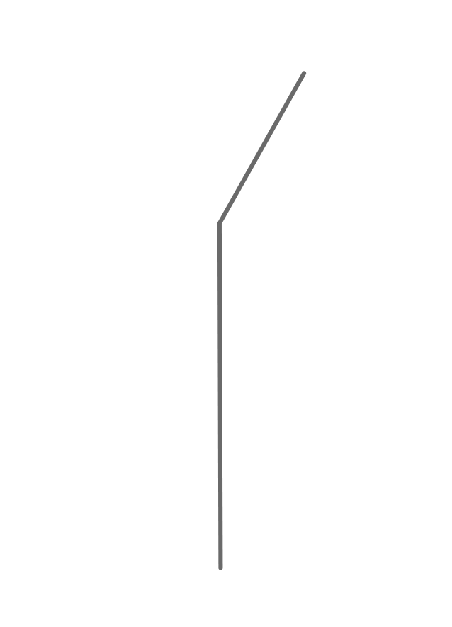
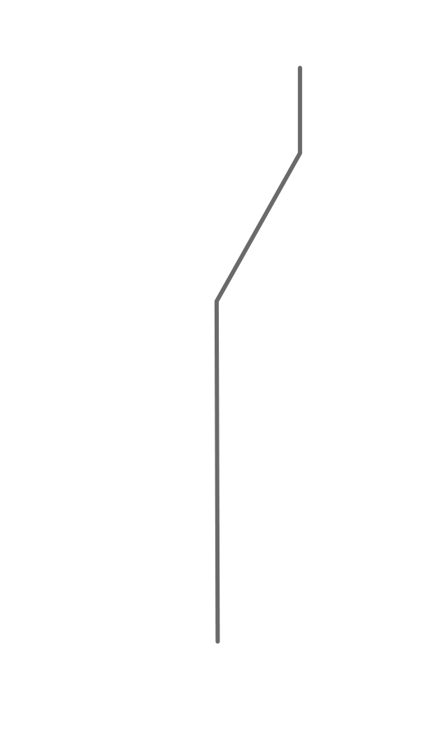
Suppose the alphabet ‘F’ represents a growth forward, forming a line.

The symbol ' + ' dictates a clockwise rotation and ' – ' dictates an anti-clockwise rotation.

Brackets [ ] represents branching.

F	F + F	F + F - F	F [ + F ] [ - F ]

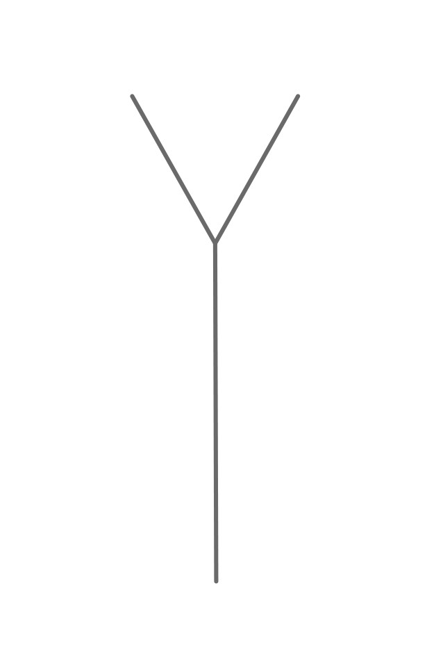Hence, the rule F → F[-F]F[F]F generates

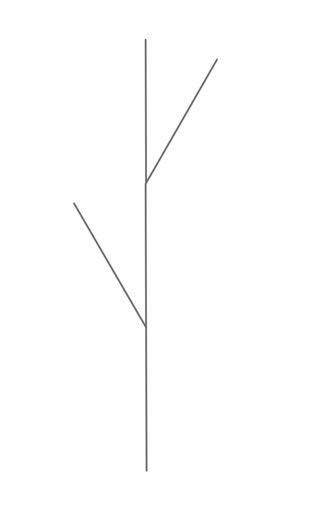
The second generation of this rule will generate

F[-F]F[+F]F[-F[-F]F[+F]F]F[-F]F[+F]F[+F[-F]F[+F]F]F[-F]F[+F]F

Which can be graphically translated into

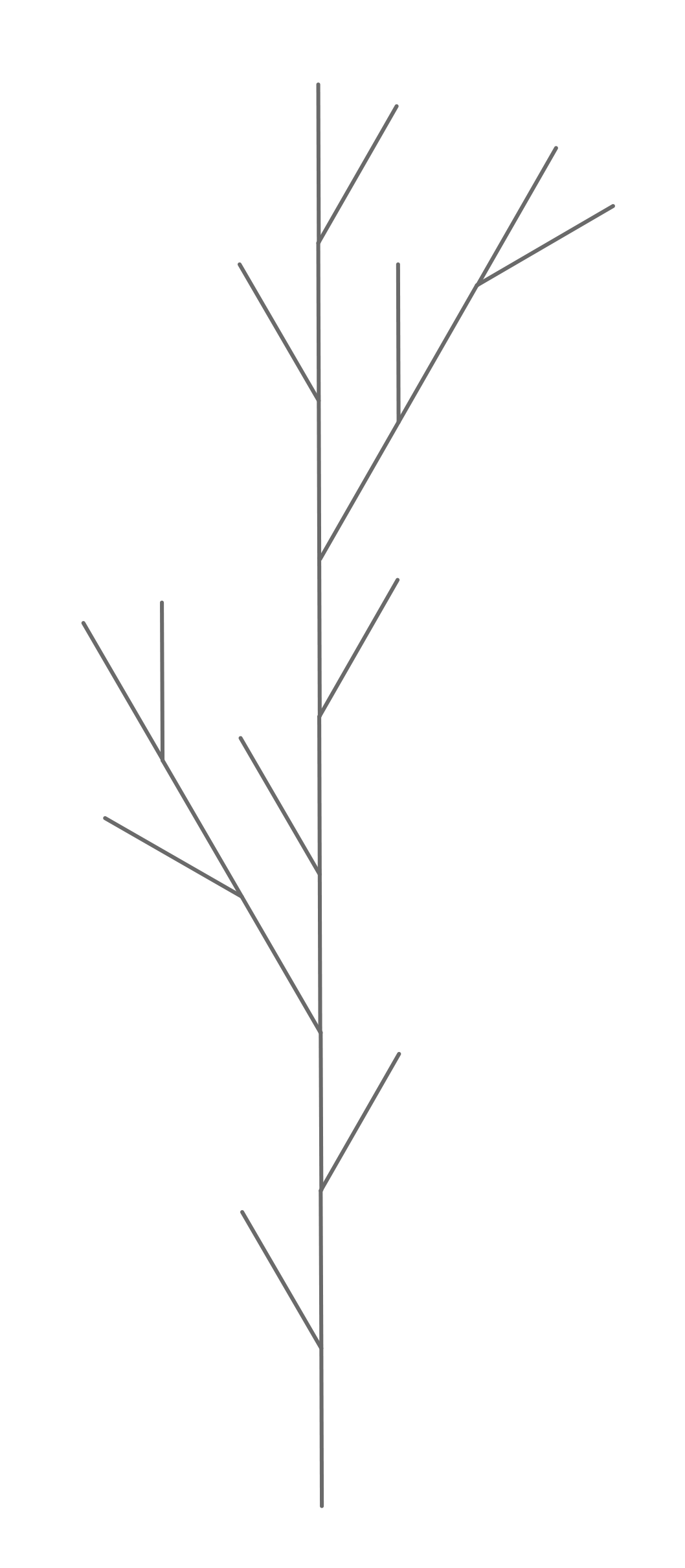
Try generating a tree with the L-systems below!

Generate Clear

Axiom: F

Rule:

Although the L-systems was first developed only to model plant growth, L-systems are now used in many design practices. Due to its robustness and tendency to form organic looking designs, the L-system has been used to solve many 2D design problems regarding roads and networks design, terrains, and textures.

Shape Grammars

A shape grammar is a “set of shape rules that can be applied to generate a set or language of designs” (Singh & Gu, 2011). Design knowledge and ideals are embedded into the grammar; hence the users of the grammar need not have the expertise in the certain design field in order to generate a design (Gu & Behbahani, 2018). Shape grammar first emerged during the 1960s, following Chomsky’s ideals on the hierarchy of formal grammars. Since then they have been studied and used in various creative fields.

The shape grammar formalism allows for algorithms to be defined directly as labelled shapes and each of these algorithms define a “language” (Stiny, 2008). According to Stiny, a shape grammar consists of four components:

• A finite set of shapes
• A finitie set of symbols
• A finite set of rules
• An initial shape

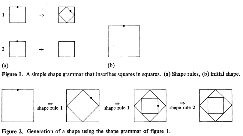
To illustrate how shape grammar works, an example from (Stiny, 2008) will be shown below.

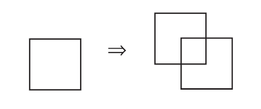
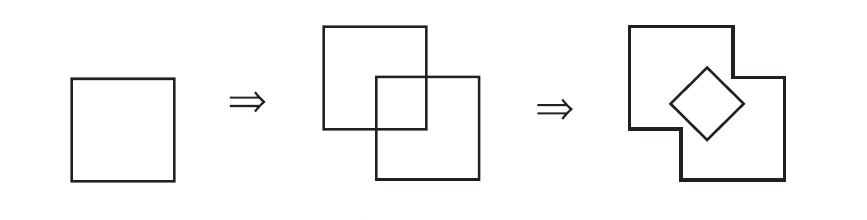
Suppose there are 2 rules dictating the transformation of a square:

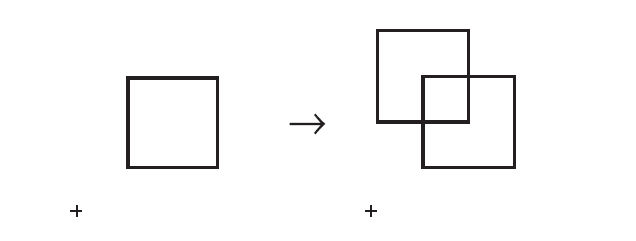
and

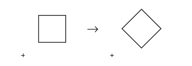
If we first apply rule 1 on a square, we will get two intersecting squares which give us two big squares and one small square as a product of the intersection.

For the next step, we can choose any of the three squares on the left-hand side (LHS) to operate on. If we choose to apply rule 2 on the small square in the middle, this is what we will get:

Another example will be of shapes labelled with symbols from (Stiny, 1980), Introduction to shape and shape grammars, which can be seen below. Rules like rule 2 below is sometimes called a termination rule since it no other rules can be applied to the shapes once the termination rule is executed.

The components and requirements for shape grammars is pretty much the same as the components and requirements for the L-system which require a set of symbols, operators, rules, and an axiom to start the system. Additionally, just like the L-systems, shape grammars can be operated in both context-free and context-sensitive conditions. For this reason, the L-system is often seen as a variation of shape grammar. Although they do share a lot of procedural similarity, they come from different linguistic concepts. While shape grammar was mainly developed from Chomsky’s idea of generative grammars (N. Gu et al., 2018), the L-system originated from string grammar which, unlike Chomsky grammars, allow for parallel rewriting (Smith, 1984). Although shape grammar allows rules to be applied in parallel as well, the rules are typically operated one at a time on matching LHS shapes, meanwhile, L-systems display multiple rule selection in each step (Gu & Behbahani, 2018). While shape grammar operates directly on the shapes themselves, the L-system operates on a string of symbols which will then produce a design.

Another difference between shape grammar and the L-system is that in the L-system all the rules are applied to any matching symbols. This is due to the symbolic nature of the L-system which will not generate unexpected outcomes. However, for shape grammar, every step might produce multiple shapes that matches the LHS shape. It is critical that all of these matching shapes are identified, yet it has been a constant challenge to date (N. Gu et al., 2018). When this happens, the designer may choose to apply the rule to every matching shape or to manually select (can be by human or computer) the emerging shapes to apply the rule to. This is even more complicated when there are more than one rules that can be applied to the specific shapes. Hence, shape grammar as a production system often requires a lot of manual intervention and is not highly automated. For this reason, shape grammars are most compatible when the design generation problem is specific and well-defined, such as for the generation of a specific housing layout.

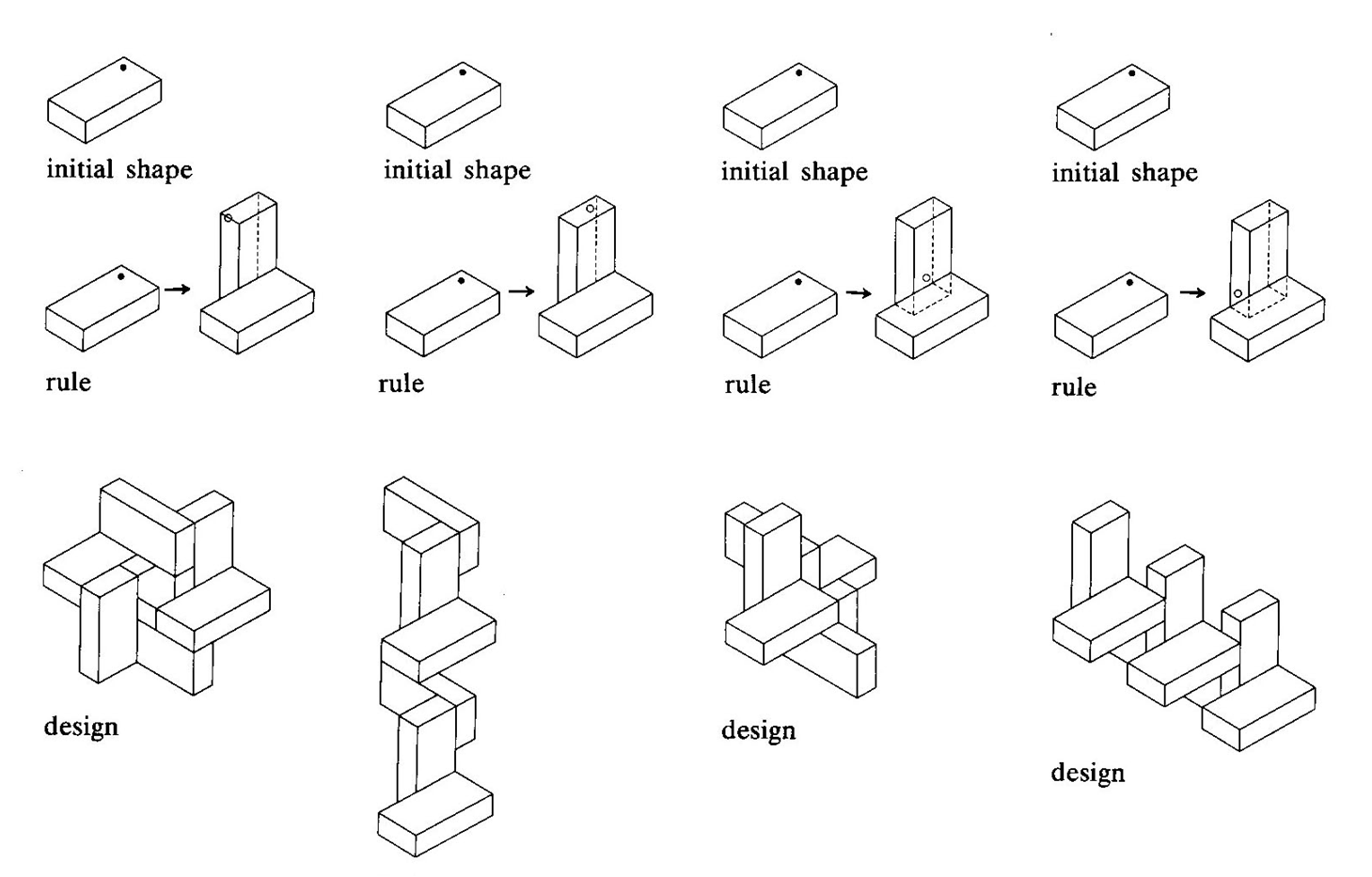
Although more complicated, shape grammar is also possible in 3D, usually for spatial exploration as shown in the example below.

Shape grammar can be used to generate new design languages or to study and understand existing design. Shape grammars are commonly used in architecture to study design typologies and styles from specific eras such as the Palladian villas (Stiny, 2008) and Chinese lattice designs (Dye, 1949). The application of shape grammar is also very useful in mass customisation of design (Duarte, 2005) as the embedded design rules significantly reduces the need for manpower in the generation stage, hence reducing cost.

Cellular Automata

A cellular automaton is a “collection of cells on a grid of a specified shaped that evolve over time according to a set of rules driven by the state of the neighbouring cells.” (Singh & Gu, 2011) Due to this dependency of each cell with its neighbouring cells, a cellular automaton is inherently context sensitive. Every cell has a state which can be binary (1 & 0, on & off, alive & dead), or non-binary (a set of colours). The rules will change the state of a certain cell depending on the current state of the concerned cell and neighbouring cells.

Although 3D cellular automata are possible, cellular automata are typically used in 1D or 2D. One-dimensional cellular automata consist of rows of cells with each row corresponding to different generations. Since the cells exist in linear rows, only left and right neighbouring cell are considered.

The sample shown above is a result of rule 222 introduced by Stephen Wolfram. At the first step, only the cell in the center is black, and then on each successive step, a cell operates according to the rules which dictate that whenever it or either of its left or right neighbours were black on the step before, the cell will be black in the next generation. Over the course of 16 generations, the system leads to a simple uniform pattern of black cells.

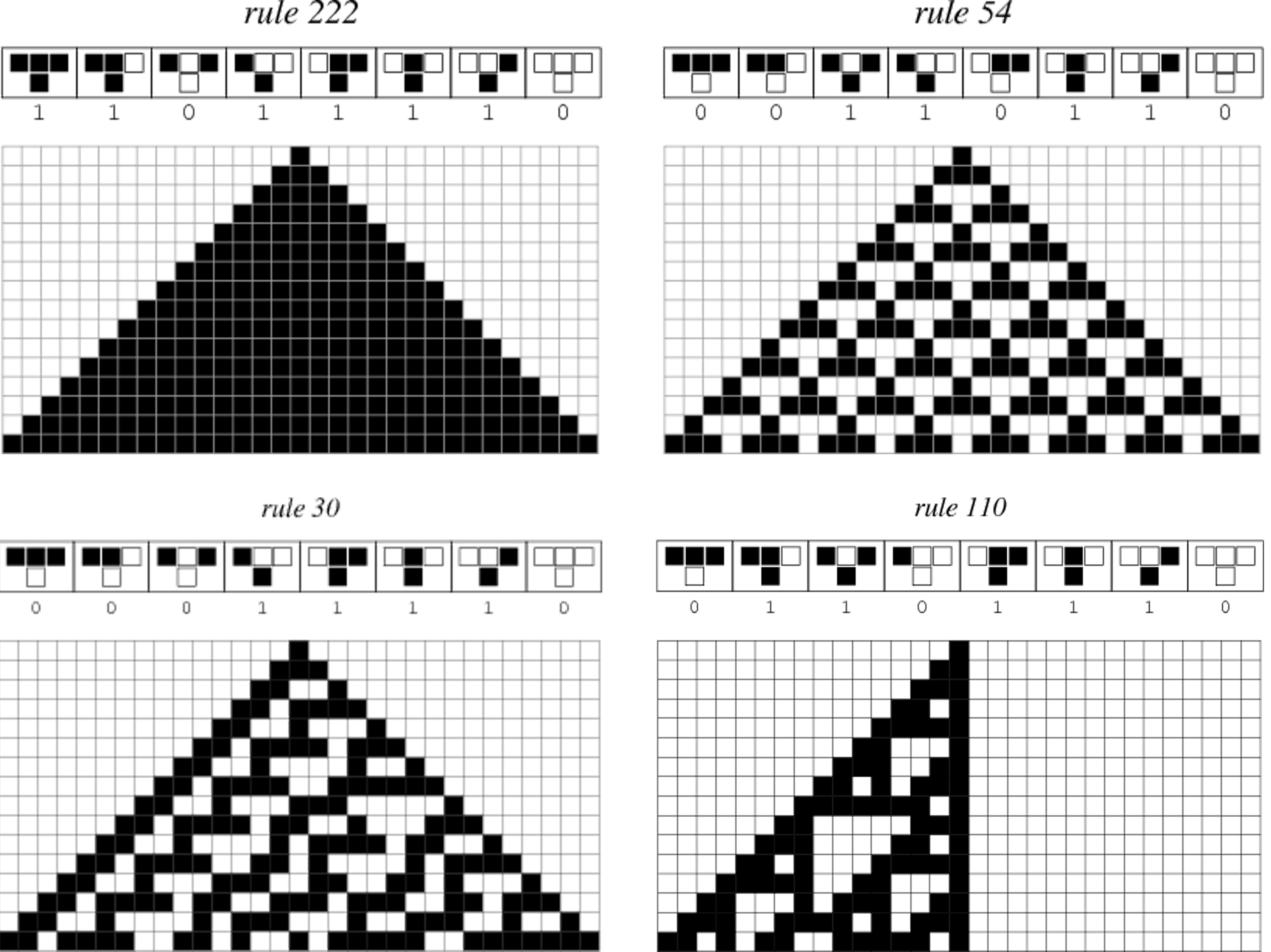
One-dimensional cellular automata can yield four different outcomes as classified by (Wolfram, 2002):

• Class 1: Cells eventually evolve into a homogeneous arrangement where every cell is the same state, never to change again. Example: Rule 222.
• Class 2: Cells form periodic patterns that endlessly cycle through a constant number of states. Example: Rule 54.
• Class 3: Cells form aperiodic, random-like patterns. Example: Rule 30.
• Class 4: Cells form a complex pattern with a localised structure that survive for a long period of time before eventually becoming either homogeneous or periodic. Example: Rule 110.

In two-dimensional cellular automata, more adjacent cells are taken into account for the rule application and not just the left and right neighbours. Below is the list of the most common 2D “neighbourhoods” (Batty, 2007).

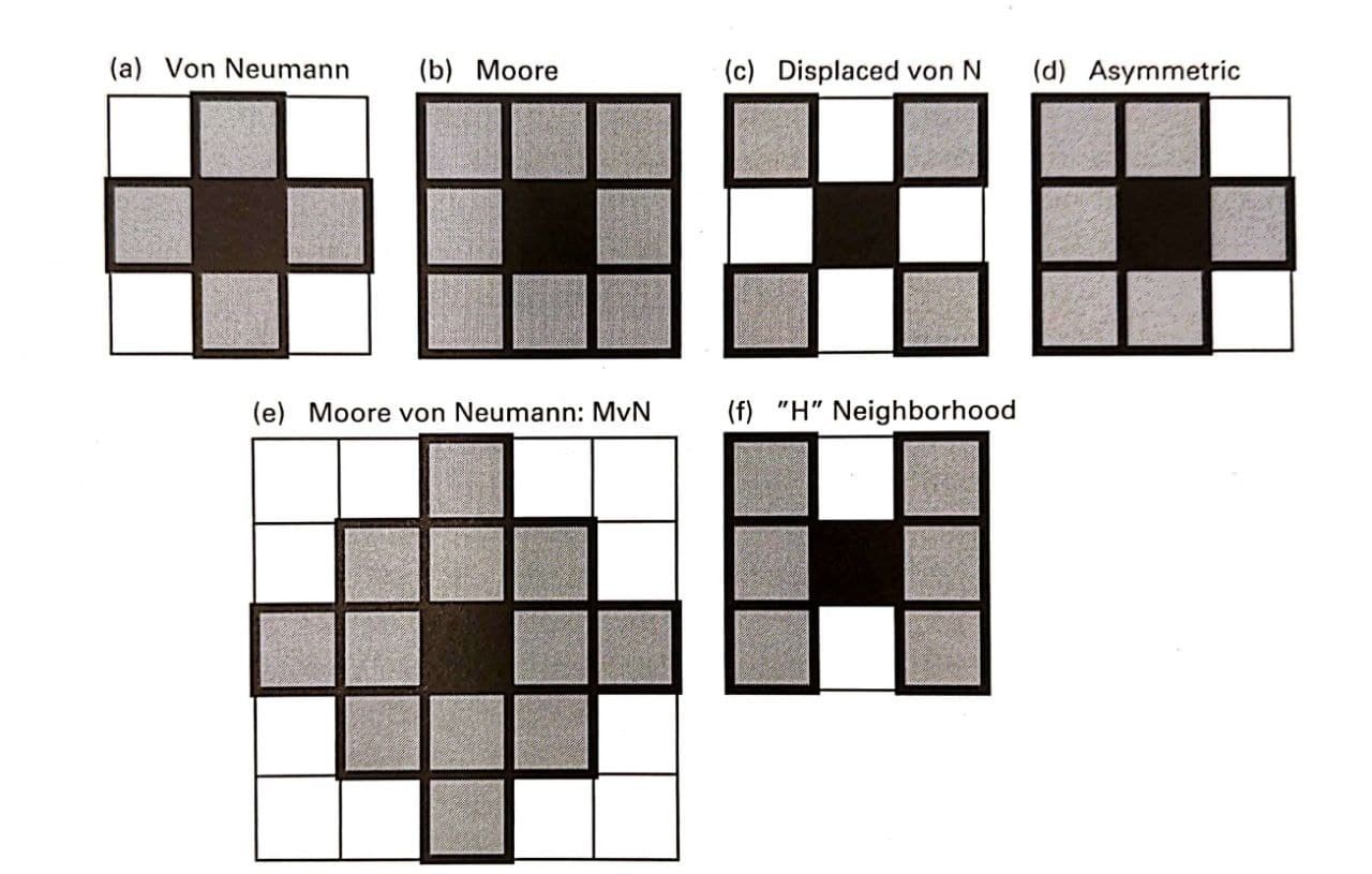
The most well-known example of a two-dimensional cellular automaton is arguably Conway’s Game of Life which operates based on the Moore neighbourhood. There are only three rules regarding the eight neighbouring cells:

• Death: If less than 2 neighbours or more than 3 neighbours are alive, the cell is dead in the next round.
• Birth: If the cell is dead and there are exactly 3 alive neighbours, the cell is alive in the next round.
• Survival: If the cell is alive and there are 2 or 3 alive neighbours, the cell remains alive in the next round.

Players start with inputting live cells into the grid (figure above) and then letting the system run on its own for as long as needed. When a pattern stabilises and does not change from one generation to another, it is known as a “still life” which is similar to the class 1 cellular automaton discussed above. When the cells form patterns that cycle through a set of configurations, they are called oscillators, and this is similar to the class 2 cellular automaton.

Try the game of life yourself below!

There are almost limitless ways to configure a cellular automaton. In the book “A New Kind of Science,” Stephen Wolfram (2002) explored “mobile automata”, where only 1 cell is active per generation; “turing machine,” which is like mobile automata, but with an added directional element; as well as “tag systems”, “substitution systems”, and many more. And those are only within the realm of one-dimensional cellular automata. As for two-dimensional cellular automata, Conway’s game of life can get even more complex and interesting when there are more parties in the game, which can be colour coded. An example of a multi-state cellular automaton on a rectangular grid with Moore neighbourhood and a rock-paper-scissors rules can be seen below.

Cellular automata systems can be used in grid based urban planning or massing. For example, Michael Batty (2007) wrote that cities should be treated as emergent structures and hence its growth can be modelled with cellular automata. Outside the design field, cellular automata can also be used to study growth patterns and social phenomenon, as can be seen from the example of Conway’s game of life. There are many variations of the traditional cellular automata system, for example, the grid used can be non-rectangular, the rules can be probabilistic, and nested cellular automata can be used to simulate more complex structures.

Attempts on Integration

Overall, each system depends on a defined set of elements that can be operated on by a defined set of production rules (Singh & Gu, 2011). Based on this similarity, many studies have been done to seek ways to integrate different systems together. For example, a study has been done by (Alfonseca, 2000) to demonstrate the equivalence of cellular automata and the L-system. They have successfully derived notations that can be used to convert even multidimensional and complicated cellular automata into L-systems. As mentioned before, it is indeed undeniable that there are a lot of overlaps between the many generative design systems and hence, different systems can be used to tackle the same problem and produce the same outputs. However, each of the different system have their own strength and weaknesses which make each one of them more suitable and efficient in tackling different problems (Singh & Gu, 2011).

In order to tap on the advantages of different systems, it is arguably more useful to combine different systems together to tackle different stages of generative design. Some examples of this would be the study done by (Stauffer & Sipper, 1998) which seeks to combine cellular automata with the L-systems and the study done in 2007 (Speller et al., 2007) where the attempt to combine cellular automata and shape grammar.

Stauffer and Sipper (1998) argued that the L-systems are naturally suited to model growth processes which means that it can also be used to model replication, which is what cellular automata are typically used for. They then devised a way to use the L-systems as the self-replicating structure and cellular automata as a way to produce graphical interpretation. By using L-systems to define the self-replication, they can make use of the simpler, linear structure of L-systems rather than the actual two or three-dimensional cellular automata implementation.

On the other hand, Speller et al. (2007) argued that both shape grammar and cellular automata approaches seek to identify a particular pattern (shape or cell) and then operate rules to transform the recognised pattern. Shape grammars requires a visual input and produces visual output that is easy for human to comprehend yet difficult for the computer to recognise. Meanwhile, a cellular automaton is computer friendly yet not intuitive for humans. Speller then claimed that by complimenting the use of cellular automata with shape grammar, a system that is both logical and can be easily programmed can be brought together with a human, intuitive approach.

Comparison & Exploration

It is apparent that the four different production systems discussed above, albeit having many similarities to one another, display different strengths and weaknesses. Each of them also has different characteristics which can be more suitable for different design scopes and purposes. The comparison of their characteristics has been summarised and tabulated below.

	Fractals	L-Systems	Shape Grammars	Cellular Automata
Components	Recursive system & initial geometry	Set of symbols, operators, rules & an axiom	Set of shapes, operators, rules & an initial shape	Cells, set of rules & initial input
Rule Application	Only one rule, one at a time	As many rules at a time, more than one at a time	One rule at a time on one matching LHS	Any relevant rules will fire when conditions are met
Context Relation	Context free	Can be context free or context sensitive	Can be context free or context sensitive	Context Sensitive
Main Characteristics	Strictly recursive, a mathematical concept	Symbolic	Geometric, visually defined	Strictly context-sensitive & bottom-up, constrained by the grid
User Involvement	Fully automated, intervention limited to initial input	Low involvement	High involvement, user chooses the shape to operate on	Fully automated, intervention limited to initial input
Purpose	Design exploration of patterns / visual compositions	Design exploration of patterns, networks & textures	Design exploration of spatial layout & To study specific architectural languages	Grid-based planning / zoning
Design Direction	Function follows form	Function follows form	Function follows form	Form follows function
Design Characteristics	Very repetitive and geometric patterns, mostly 2D	Repetitive patterns that tend to be organic, mostly 2D	Geometric shapes, can be 2D and 3D	Grid constrained outcomes, typically 2D

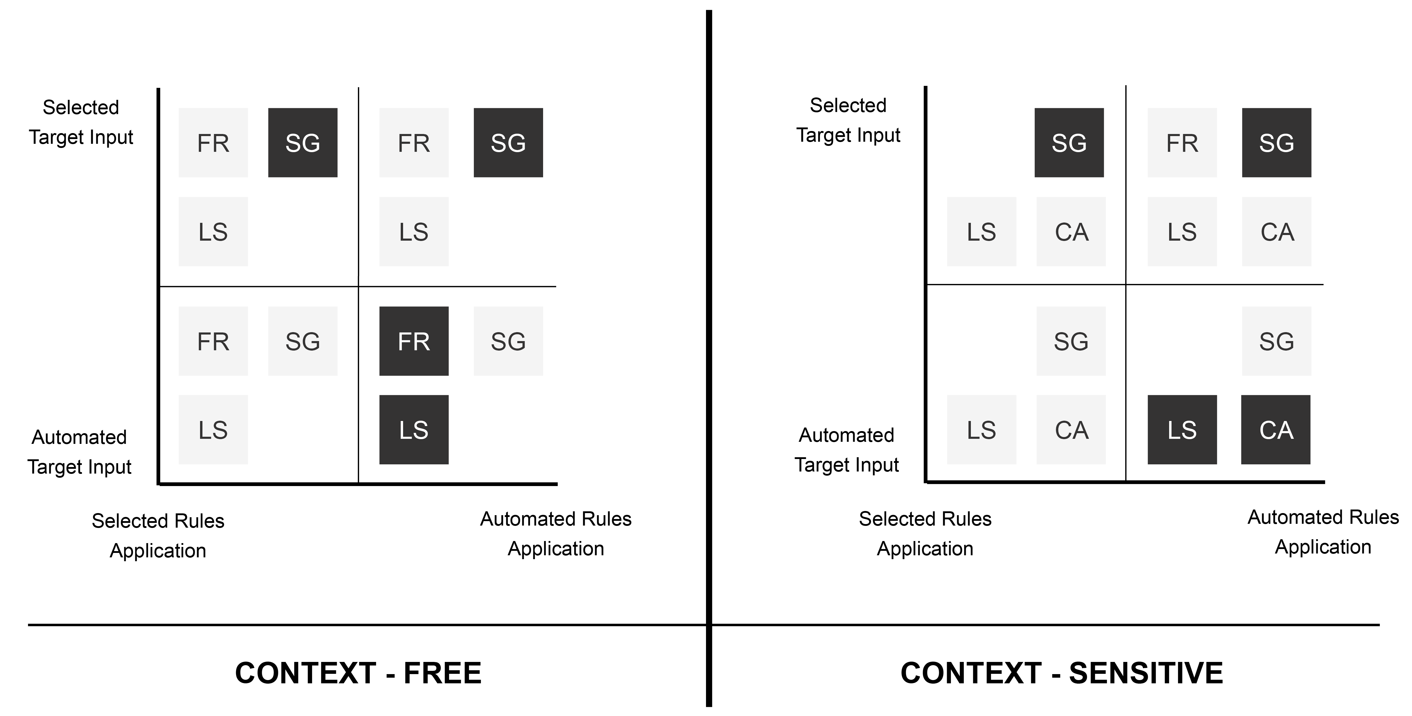
As mentioned in the introduction, this paper seeks to explore a different way of integrating these different systems by using one system as an input element of another. To do this, first, the four different systems will be studied in more depth by comparing them in a single matrix. From the table above, only the rule application and context relation elements will be integrated in the matrix since the focus is not on the design purpose, but on the generative nature of the systems.

Three different input aspects will be compiled in a matrix as a means to compare the four systems and examine the relationship between them. The three aspects are:

• Context-free VS Context-sensitive
• Selected rules application VS Automated rules application
• Selected target input VS Automated target input

Context-sensitive systems means that the matching LHS target depend on the condition of its surrounding, for example, a cellular automaton is inherently context-sensitive as the target input depends on the state of the neighbouring cells. The rules application applies to cases where there are multiple rules targeted at the same input while the target input applies to the context where there are multiple matching LHS inputs. The four systems, fractals (FR), L-systems (LS), shape grammars (SG), and cellular automata (CA) have been categorised into the matrix shown below. The dark ones show the typical region where the system lays in the matrix while the light ones represents where the system is feasible but not commonly used. For example, there is typically only one rule used per L-system and the system will generate a recursive geometry with only one rule. However, the L-system example provided in the section above lets the user change the rule applied between generations, making it possible to generate more complex tree structures.

To integrate a production system as an input of another, the different inputs and outputs of the systems must also be investigated. The following diagram describes the characteristics of the inputs and outputs of the four different systems and the compatibility between them.

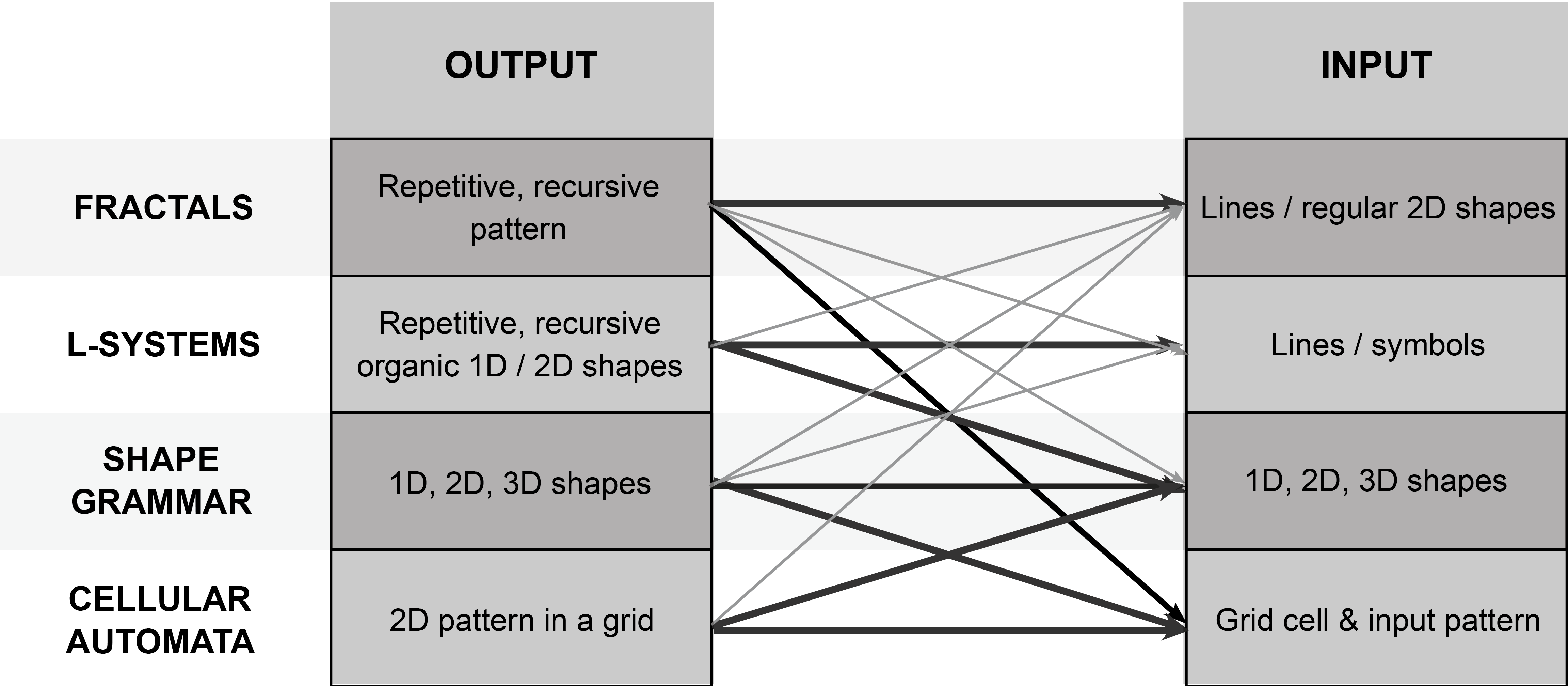
From the diagram above, it can be seen that most systems can produce an output that can serve as an input for another. However, some connections (notated with the thicker arrows) are stronger than the rest. The connection in thin arrows denotes outputs that either might not always match the input of the second system, might not produce a notably different system or might be terminative to the system.

Excluding the cases where the same system inputs to itself, when the possibility of both automated system and system with manual selection is considered, the strong connections are:

• Fractals → Cellular Automata
• L-systems → Shape Grammars
• Shape Grammars → Cellular Automata
• Cellular Automata → Shape Grammars

Using the recursive nature of fractals, a regular or nested grid can be produced for a cellular automaton, meanwhile, a shape grammar system can be used to divide a plot into an irregular grid of cells for a cellular automaton. Irregular grids can be very useful for the use of a cellular automaton in urban planning context (Pinto et al., 2017). On the other hand, both a regular and irregular grid cellular automaton produce patterns that can serve as input shapes for a shape grammar system. This could again, be useful for urban planning context, or to automatically generate a city model. The shape grammar can be used for a smaller scaled spatial layout division or to generate buildings on the plots of land (cells). Lastly, an L-system can be used to generate an organic network which will serve as an input for a shape grammar system which will then further operate on the matching LHS.

It is also possible to use the different systems back and forth or sequentially depending on the context. For example, it is possible to use:

Fractals → Cellular Automata → Cellular Automata → Shape Grammars

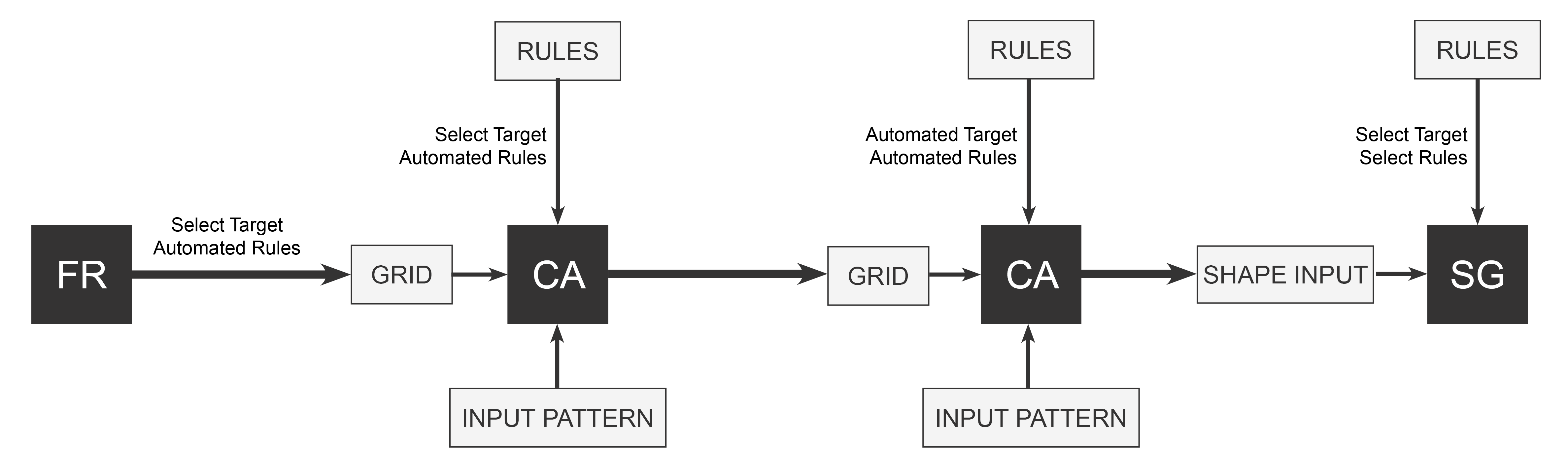
Based on the flowchart above, a fractal system can first be used to divide a plot into smaller grids, creating a nested grid as per the users’ wish since it allows target selection. This grid will then be fed as a cell for a cellular automaton where the user can define the input pattern. Two rounds of cellular automata can be done where the first allow target selection for the user to solve the nested cells first before then solving the entire grid with an automated system. The patterns generated can then be used as shape inputs for a shape grammar system which will then sub divide them into smaller plots. This system can be used for complex systems and irregular cells generation for acellular automata. As a proof of concept, a very simple example will be displayed below.

First, a Peano curve fractal system is used to divide a square plot into smaller squares. Target selection is enabled, hence allowing users to create nested cells as such.

One of the nested grids is selected for the first round of cellular automaton. The system used here is a simple three-coloured rock-paper-scissors system. A random input pattern is generated to start the cellular automaton and is stopped after five generations.

The other nested grids are filled and the colour with the greatest number of cells in each grid is taken as the representative colour of the parent cell. These three cells are frozen, meaning that they will not change colour although their colours will affect the colours of their neighbouring cells. The same rock-paper-scissors system is run with another random input pattern. The cellular automaton is again stopped after five generations.

Before moving on to apply a shape grammar system on the resultant pattern, a set of simple shape grammar rules are defined below.

Matching shapes from particular-coloured cells are recognised and selected for the shape grammar operation.

User can select both the target and rules as the wish.

After six generations of shape grammar operations, the plot division is finished and the result can be seen below. The resultant geometry displays a robust plot division. The integration of the fractal system enables exploration in different scales within the cellular automaton. Meanwhile, the shape grammar system introduces more irregular geometries into the plot, breaking the repetitiveness of a cellular automata’s grid, and resulting in a less rigid plot division.

Conclusion

Today, there are plenty of available generative design systems and it is unavoidable that their use and methods overlap a lot with one another. It is then inevitable that these similarities in methods, language, input, or output confuses many and prevent a clear boundary between the systems to be defined.

This essay has reviewed four different production systems to closely examine the differences and similarities between them before then proposing a way to integrate different production systems. The proposed way of integration is done by using the output of one system as an input of another. A simple example has been demonstrated in the previous section where a chain of different production systems is operated sequentially to divide a rectangular plot. The resultant geometry of the divided plot looks arguably intriguing. However, the focus of this essay is to integrate the systems based on their generative nature; hence the functionality of the proposed method has not been investigated. Future work may include studying the practicality of the proposed method in serving a specific design purpose.

References

Alfonseca, M., & Ortega, A. (1996). Representation of fractal curves by means of L Systems. Proceedings of the Conference on Designing the Future - APL '96. doi:10.1145/253341.253348

Alfonseca, Manuel & De la Puente, Alfonso. (2000). Representation of some cellular automata by means of equivalent L Systems. Complexity. 7.

Batty, M. (2007). Cities and complexity: Understanding cities with cellular automata, agent-based models and fractals. Cambridge, MA: MIT Press.

Duarte, Jose. (2005). Customizing mass housing : a discursive grammar for Siza's Malagueira houses. Massachusetts Institute of Technology. Dept. of Architecture.

Dye, D. S. (1949). A grammar of Chinese lattice. Cambridge, MA: Harvard University Press.

Flake, W. (2000). Computational beauty of nature. Cambridge, MA: MIT Press.

Gu, N., & Behbahani, P. A. (2018). Shape grammars: A key generative design algorithm. Handbook of the Mathematics of the Arts and Sciences, 1-21. doi:10.1007/978-3-319-70658-0_7-1

Gu, N., Yu, R., & Behbahani, P. A. (2018). Parametric design: Theoretical development and Algorithmic foundation for DESIGN generation in architecture. Handbook of the Mathematics of the Arts and Sciences, 1-22. doi:10.1007/978-3-319-70658-0_8-1

Mandelbrot, B. B. (1983). The fractal geometry of nature. New York: Freeman.

Pinto, N., Antunes, A. P., & Roca, J. (2017). Applicability and calibration of an irregular cellular automata model for land use change. Computers, Environment and Urban Systems, 65, 93-102. doi:10.1016/j.compenvurbsys.2017.05.005

Prusinkiewicz, P., & Lindenmayer, A. (1996). The algorithmic beauty of plants. New York: Springer-Verlag.

Sedrez, M. R., & Cybis Pereira, A. T. (2012). Fractal shape. Architecture, Systems Research and Computational Sciences, 97-107. doi:10.1007/978-3-0348-0393-9_8

Shiffman, D. (2012). The nature of code simulating natural systems with processing. Erscheinungsort nicht ermittelbar: Selbstverl.

Singh, V., & Gu, N. (2012). Towards an integrated generative design framework. Design Studies, 33(2), 185-207. doi:10.1016/j.destud.2011.06.001

Smith, A. R. (1984). Plants, fractals, and formal languages. Proceedings of the 11th Annual Conference on Computer Graphics and Interactive Techniques - SIGGRAPH '84. doi:10.1145/800031.808571

Speller, Thomas & Whitney, Daniel & Crawley, Edward. (2007). Using shape grammar to derive cellular automata rule patterns. Complex Systems. 17.

Stauffer, A., & Sipper, M. (1998). On the relationship between cellular automata and l-systems: The self-replication case. Physica D: Nonlinear Phenomena, 116(1-2), 71-80. doi:10.1016/s0167-2789(97)00255-8

Stiny, G. (1980). Introduction to shape and shape grammars. Environment and Planning B: Planning and Design, 7(3), 343-351. doi:10.1068/b070343

Stiny, G. (2008). Shape: Talking about seeing and doing. Cambridge, MA: MIT.

Vaughan, J., & Ostwald, M. J. (2018). Fractal geometry in architecture. Handbook of the Mathematics of the Arts and Sciences, 1-16. doi:10.1007/978-3-319-70658-0_11-1

Wolfram, S. (2002). A new kind of science. México: Wolper production.